直方图是图像处理过程中的一种非常重要的分析工具。直方图从图像内部灰度级的角度对图像进行表述,包含十分丰富而重要的信息。从直方图的角度对图像进行处理,可以达到增强图像显示效果的目的。
在绘制直方图时,将灰度级作为x轴,该灰度出现的次数作为y轴处理。
绘制直方图
使用Numpy绘制直方图
1
2
3
4
| import cv2
from get_show_img import get_show
o = cv2.imread('data/dog1.jpg')
get_show(o, figsize=[6, 6])
|

1
2
3
| import matplotlib.pyplot as plt
plt.hist(o.ravel(), 256)
plt.show()
|
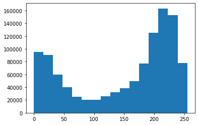
将灰度级划分为16组。
1
2
| plt.hist(o.ravel(), 16)
plt.show()
|
使用opencv绘制直方图
cv2.calcHist(images, channels, mask, histSize, ranges, accumulate)
- images: 原始图像,该图像需要用[]括起来。
- channels: 指定的通道编号. 通道编号用[]括起来,灰度图像对应[0],彩色图像R、G、B分别对应[0]、[1]、[2]。
- mask: 掩膜图像。当统计整幅图像时,设定为None。
- histSize: BINS的值,该值需要用[]括起来。
- ranges: 像素范围。
- accumulate: 累计(累积、叠加)标识,默认值为False。如果被设置为True,则直方图在开始计算时不会被清零,计算的是多个直方图的累积结果,用于对一组图像计算直方图。
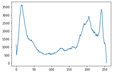
1
| hist = cv2.calcHist([o], [0], None, [256], [0, 255])
|
(256, 1)
256
<class 'numpy.ndarray'>
1
2
| plt.plot(hist)
plt.show()
|
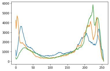
将多个通道的直方图绘制到一幅图像中
1
2
3
| hist0 = cv2.calcHist([o], [0], None, [256], [0, 255])
hist1 = cv2.calcHist([o], [1], None, [256], [0, 255])
hist2 = cv2.calcHist([o], [2], None, [256], [0, 255])
|
1
2
3
4
| plt.plot(hist0)
plt.plot(hist1)
plt.plot(hist2)
plt.show()
|
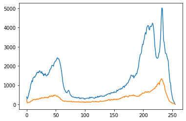
使用掩膜图像绘制直方图
1
2
| img = cv2.imread('data/dog1.jpg', 0)
mask = np.zeros_like(img)
|
1
| mask[200:500, 200:500] = 255
|
1
2
3
4
5
| hist = cv2.calcHist([img], [0],None, [256], [0, 255])
hist_mask = cv2.calcHist([img], [0], mask, [256], [0, 255])
plt.plot(hist)
plt.plot(hist_mask)
plt.show()
|
直方图均衡化
如果一幅图像拥有全部可能的灰度级,并且像素值的灰度均匀分布,那么这幅图像就具有高对比度和多变的灰色色调,灰度级丰富且覆盖范围较大。在外观上,这样的图像具有更丰富的色彩,不会过暗或者过亮。
1
2
3
| eq1 = cv2.imread('data/equ.bmp', 0)
eq2 = cv2.imread('data/equ2.bmp', 0)
get_show(eq1, eq2)
|

1
2
| equ1 = cv2.equalizeHist(eq1)
get_show(eq1, equ1)
|

1
2
| equ2 = cv2.equalizeHist(eq2)
get_show(eq2, equ2)
|

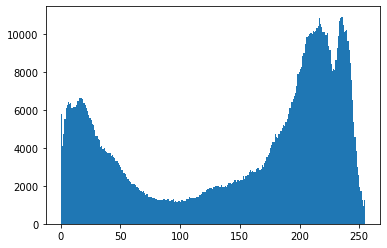
1
2
3
4
5
| hist1 = cv2.calcHist([eq2], [0], None, [256], [0, 255])
hist2 = cv2.calcHist([equ2], [0], None, [256], [0, 255])
plt.plot(hist1)
plt.plot(hist2)
plt.show()
|
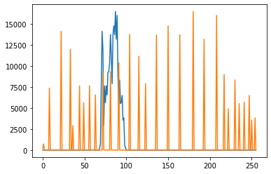
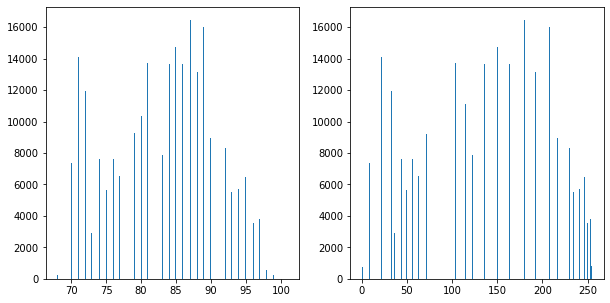
1
2
3
4
5
6
| plt.figure(figsize=[10, 5])
plt.subplot(121)
plt.hist(eq2.ravel(), 256)
plt.subplot(122)
plt.hist(equ2.ravel(), 256)
plt.show()
|