任务1

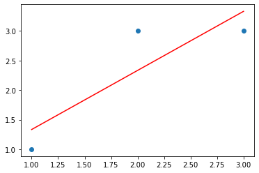
求出利用最小二乘法通过(1,1) (2,3) (3,3)三点拟合出的直线 # b = 0.1 a = 1.1

$y=wx + b$

创建数据

1	import numpy as np

1
2
3

# sklearn中要求自变量（特征）的维度是二维
x = np.array([[1], [2], [3]])
y = np.array([1, 3, 3])

模型的建立和训练

# 导入回归模型
# LinearRegression: 线性回归模型
# LogisticRegression: 逻辑回归模型
# LogisticRegressionCV: 逻辑回归模型引入交叉验证默认是10折交叉验证
from sklearn.linear_model import LinearRegression, LogisticRegression, LogisticRegressionCV
# 决策树模型
# DecisionTreeClassifier: 决策树分类模型
# DecisionTreeRegressor: 决策树回归模型
from sklearn.tree import DecisionTreeClassifier, DecisionTreeRegressor
# 支持向量机
# SVC: 支持向量机分类模型
# SVR: 支持向量机回归模型
from sklearn.svm import SVC, SVR
# 神经网络模型
# MLPClassifier: 神经网络分类模型
# MLPRegressor: 神经网络回归模型
from sklearn.neural_network import MLPClassifier, MLPRegressor
# 聚类模型
# KMeans: K均值聚类模型
# DBSCAN: 密度聚类
from sklearn.cluster import KMeans, DBSCAN
# 朴素贝叶斯模型
from sklearn.naive_bayes import BaseEstimator
# 随机森林模型
# RandomForestClassifier: 随机森林分类模型
# RandomForestRegressor: 随机森岭回归模型
from sklearn.ensemble import RandomForestClassifier, RandomForestRegressor

# 进行模型的实例化
linear_model = LinearRegression()

# 模型的训练
linear_model.fit(x, y)

LinearRegression()

查看模型参数

1 2	# 查看模型的权重 linear_model.coef_

array([1.])

1 2	# 查看模型的截距 linear_model.intercept_

0.33333333333333437

1 2	# 获取构造方法的参数信息 linear_model.get_params()

{'copy_X': True,
 'fit_intercept': True,
 'n_jobs': None,
 'normalize': 'deprecated',
 'positive': False}

模型预测

1
2
3

# 使用模型进行预测
y_pre = linear_model.predict(x)
y_pre

array([1.33333333, 2.33333333, 3.33333333])

可视化

import matplotlib.pyplot as plt

# 绘制散点图和模型预测结果
plt.scatter(x, y)
plt.plot(x, y_pre, c='r')
plt.show()

任务2

输入：[[0, 0], [1, 1], [2, 2]]——两个输入

输出：[0, 1, 2]

预测：[3, 3]

$y=w_1x_1 + w_2x_2 + b$

创建数据

1 2	x = np.array([[0, 0], [1, 1], [2, 2]]) y = np.array([0, 1, 2])

模型的建立和训练

1	from sklearn.linear_model import LinearRegression

1 2	# 模型实例化 linear_model2 = LinearRegression(fit_intercept=False)

1 2	# 模型的训练 linear_model2.fit(x, y)

LinearRegression(fit_intercept=False)

查看模型的参数

1	linear_model2.coef_

array([0.5, 0.5])

1	linear_model2.intercept_

0.0

模型预测

1 2	# 预测特征也必须是二维的 x_test = np.array([[3, 3]])

1	linear_model2.predict(x_test)

array([3.])

任务3:波士顿房价预测

获取数据/读取数据

1 2	# 导入sklean内置数据集 from sklearn.datasets import load_boston

data: 特征值
target: 标签值
feature_names: 特征名称
DESCR: 数据集的描述信息
filename: 导入的数据文件名称
data_module: 数据集所在模块

1 2	# 获取的数据被保存在一个字典中 data = load_boston()

1
2
3

x = data['data']
y = data['target']
x_name = data['feature_names']

1	print(x.shape)

(506, 13)

1	print(y.shape)

(506,)

数据探索

for i in range(x.shape[1]):
    tmp_x = x[:, i]
    plt.scatter(tmp_x, y, s=10)
    plt.title(f'y~{x_name[i]}')
    plt.show()

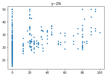
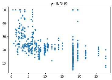
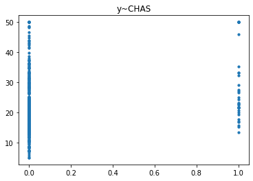
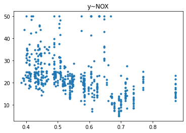
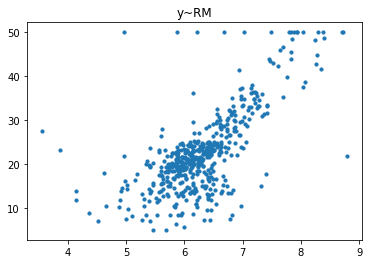
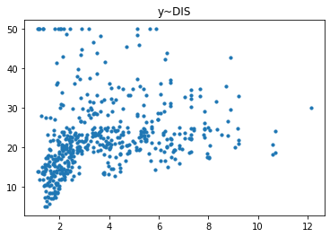
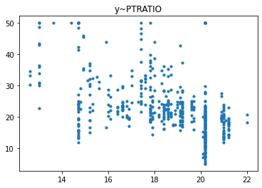
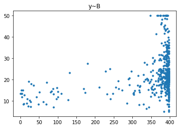
经过对散点图的观测，我们发现只有RM和LSTAT这两列与房价有比较强的相关关系，一个是正相关一个是负相关，所以后续的研究我们以RM这列作为研究对象，预测其与房价的回归模型。

数据的预处理

1
2
3

# 将RM列单独取出
x = x[:, 5:6]
# 注意：要保持原始数据的二维结构，在取数据时必须使用切片方式

# 数据集的切分
# 使用留出法将数据集切分为训练集和测试集
from sklearn.model_selection import train_test_split

x_train, x_test, y_train, y_test = train_test_split(x, y, test_size=0.2)
print(x_train.shape)
print(x_test.shape)

(404, 1)
(102, 1)

模型的建立和训练

1	from sklearn.linear_model import LinearRegression

1	linear_model3 = LinearRegression()

1	linear_model3.fit(x_train, y_train)

LinearRegression()

查看模型参数

1	linear_model3.coef_

array([9.12377512])

1	linear_model3.intercept_

-34.702321066310034

模型的预测

1	y_pred = linear_model3.predict(x_test)

可视化预测直线

1
2
3

plt.scatter(x_test, y_test)
plt.plot(x_test, y_pred, c='r')
plt.show()

模型的评价

回归模型的默认评价指标是$R^2$

1	linear_model3.score(x_test, y_test)

0.41700102985892673

r2_score: $R^2$值(拟合优度)
mean_squared_error: 均方误差(MSE)

1	from sklearn.metrics import r2_score, mean_squared_error

1	r2_score(y_test, y_pred)

0.41700102985892673

1	mean_squared_error(y_test, y_pred)

50.85450032392045

任务4：研究生录取预测

数据集下载

读取数据

1	import pandas as pd

1 2	data = pd.read_csv('LogisticRegression.csv') data

	admit	gre	gpa	rank
0	0	380	3.61	3
1	1	660	3.67	3
2	1	800	4.00	1
3	1	640	3.19	4
4	0	520	2.93	4
...	...	...	...	...
395	0	620	4.00	2
396	0	560	3.04	3
397	0	460	2.63	2
398	0	700	3.65	2
399	0	600	3.89	3

400 rows × 4 columns

数据探索

重复值处理

1 2	# 去出重复值前的尺寸 data.shape

(400, 4)

1 2	# 去除重复值操作 data.drop_duplicates(inplace=True)

1 2	# 去出重复值后的尺寸 data.shape

(395, 4)

说明数据集存在5条重复数据

缺失值探索

1	data.isna().sum()

admit    0
gre      0
gpa      0
rank     0
dtype: int64

说明数据框中不存在缺失值

数据预处理

1
2
3

# 分离特征和标签
x = data.iloc[:, -3:]
y = data.iloc[:, 0]

1 2	print(x.shape) print(y.shape)

(395, 3)
(395,)

# 数据集的切分
# 使用留出法将数据集切分为训练集和测试集
from sklearn.model_selection import train_test_split

x_train, x_test, y_train, y_test = train_test_split(x, y, test_size=0.2)
print(x_train.shape)
print(x_test.shape)

(316, 3)
(79, 3)

模型的建立和训练

1	from sklearn.linear_model import LogisticRegression

1	logistic_model = LogisticRegression()

1	logistic_model.fit(x_train, y_train)

LogisticRegression()

模型的预测

1	y_pred = logistic_model.predict(x_test)

模型的评价

1 2	# 在Sklearn中分类模型的评价指标默认是accuracy logistic_model.score(x_test, y_test)

0.759493670886076

1 2	# 精确度 from sklearn.metrics import accuracy_score

1	accuracy_score(y_test, y_pred)

0.759493670886076

# 查准率
from sklearn.metrics import precision_score

precision_score(y_test, y_pred)

0.8888888888888888

# 查全率
from sklearn.metrics import recall_score

recall_score(y_test, y_pred)

0.3076923076923077

# f1值
from sklearn.metrics import f1_score

f1_score(y_test, y_pred)

0.4571428571428572

# 打印分类报告（包含精确率、查准率、查全率、F1值）
from sklearn.metrics import classification_report

print(classification_report(y_test, y_pred))

              precision    recall  f1-score   support

           0       0.74      0.98      0.85        53
           1       0.89      0.31      0.46        26

    accuracy                           0.76        79
   macro avg       0.82      0.64      0.65        79
weighted avg       0.79      0.76      0.72        79

Ming-Log's Blog

Python数据科学_7_回归分析基础

任务1

创建数据

模型的建立和训练

查看模型参数

模型预测

可视化

任务2

创建数据

模型的建立和训练

查看模型的参数

模型预测

任务3:波士顿房价预测

获取数据/读取数据

数据探索

数据的预处理

模型的建立和训练

查看模型参数

模型的预测

可视化预测直线

模型的评价

任务4：研究生录取预测

读取数据

数据探索

重复值处理

缺失值探索

数据预处理

模型的建立和训练

模型的预测

模型的评价