目标:
求出现有的13个特征中,哪几个特征对y(地方财政收入)影响最大
求出2014年和2015年这两年的财政收入
数据集下载
读取数据 1 2 data = pd.read_csv('data.csv' , index_col=0 ) data.head()
x1
x2
x3
x4
x5
x6
x7
x8
x9
x10
x11
x12
x13
y
1994.0
3831732.0
181.54
448.19
7571.00
6212.70
6370241.0
525.71
985.31
60.62
65.66
120.0
1.029
5321.0
64.87
1995.0
3913824.0
214.63
549.97
9038.16
7601.73
6467115.0
618.25
1259.20
73.46
95.46
113.5
1.051
6529.0
99.75
1996.0
3928907.0
239.56
686.44
9905.31
8092.82
6560508.0
638.94
1468.06
81.16
81.16
108.2
1.064
7008.0
88.11
1997.0
4282130.0
261.58
802.59
10444.60
8767.98
6664862.0
656.58
1678.12
85.72
91.70
102.2
1.092
7694.0
106.07
1998.0
4453911.0
283.14
904.57
11255.70
9422.33
6741400.0
758.83
1893.52
88.88
114.61
97.7
1.200
8027.0
137.32
数据探索 <class 'pandas.core.frame.DataFrame'>
Float64Index: 22 entries, 1994.0 to nan
Data columns (total 14 columns):
# Column Non-Null Count Dtype
--- ------ -------------- -----
0 x1 20 non-null float64
1 x2 20 non-null float64
2 x3 20 non-null float64
3 x4 20 non-null float64
4 x5 20 non-null float64
5 x6 20 non-null float64
6 x7 20 non-null float64
7 x8 20 non-null float64
8 x9 20 non-null float64
9 x10 20 non-null float64
10 x11 20 non-null float64
11 x12 20 non-null float64
12 x13 20 non-null float64
13 y 20 non-null float64
dtypes: float64(14)
memory usage: 2.6 KB
可见该数据集无缺失值和类别型特征
数据预处理 将数据集的特征和标签分离 1 2 x = data.iloc[:-2 , :-1 ] y = data.iloc[:-2 , -1 :]
筛选重要特征
案例,方案有要求,需要筛选出重要特征
当数据中特征数量比较多的时候,会需要去筛选出重要特征。
1 2 from sklearn.linear_model import Lasso
1 2 3 4 5 6 7 alpha = 10000 lasso_model = Lasso(alpha=alpha) lasso_model.fit(x, y) feature_num = np.sum (lasso_model.coef_ != 0 ) new_feature = x.columns[lasso_model.coef_ != 0 ] print (f'alpha={alpha} , 特征数={feature_num} ' )print ('新特征为:' , new_feature)
alpha=10000, 特征数=5
新特征为: Index(['x1', 'x4', 'x5', 'x6', 'x13'], dtype='object')
D:\Users\Python\Anaconda3.8\lib\site-packages\sklearn\linear_model\_coordinate_descent.py:647: ConvergenceWarning: Objective did not converge. You might want to increase the number of iterations, check the scale of the features or consider increasing regularisation. Duality gap: 5.937e+04, tolerance: 7.053e+02
model = cd_fast.enet_coordinate_descent(
1 new_x = x.loc[:, new_feature]
x1
x4
x5
x6
x13
1994.0
3831732.0
7571.00
6212.70
6370241.0
5321.0
1995.0
3913824.0
9038.16
7601.73
6467115.0
6529.0
1996.0
3928907.0
9905.31
8092.82
6560508.0
7008.0
1997.0
4282130.0
10444.60
8767.98
6664862.0
7694.0
1998.0
4453911.0
11255.70
9422.33
6741400.0
8027.0
1999.0
4548852.0
12018.52
9751.44
6850024.0
8549.0
2000.0
4962579.0
13966.53
11349.47
7006896.0
9566.0
2001.0
5029338.0
14694.00
11467.35
7125979.0
10473.0
2002.0
5070216.0
13380.47
10671.78
7206229.0
11469.0
2003.0
5210706.0
15002.59
11570.58
7251888.0
12360.0
2004.0
5407087.0
16884.16
13120.83
7376720.0
14174.0
2005.0
5744550.0
18287.24
14468.24
7505322.0
16394.0
2006.0
5994973.0
19850.66
15444.93
7607220.0
17881.0
2007.0
6236312.0
22469.22
18951.32
7734787.0
20058.0
2008.0
6529045.0
25316.72
20835.95
7841695.0
22114.0
2009.0
6791495.0
27609.59
22820.89
7946154.0
24190.0
2010.0
7110695.0
30658.49
25011.61
8061370.0
29549.0
2011.0
7431755.0
34438.08
28209.74
8145797.0
34214.0
2012.0
7512997.0
38053.52
30490.44
8222969.0
37934.0
2013.0
7599295.0
42049.14
33156.83
8323096.0
41972.0
求2014年和2015年的财政收入 1 2 new_x.loc[2014 , :] = np.NAN new_x.loc[2015 , :] = np.NAN
x1
x4
x5
x6
x13
1994.0
3831732.0
7571.00
6212.70
6370241.0
5321.0
1995.0
3913824.0
9038.16
7601.73
6467115.0
6529.0
1996.0
3928907.0
9905.31
8092.82
6560508.0
7008.0
1997.0
4282130.0
10444.60
8767.98
6664862.0
7694.0
1998.0
4453911.0
11255.70
9422.33
6741400.0
8027.0
1999.0
4548852.0
12018.52
9751.44
6850024.0
8549.0
2000.0
4962579.0
13966.53
11349.47
7006896.0
9566.0
2001.0
5029338.0
14694.00
11467.35
7125979.0
10473.0
2002.0
5070216.0
13380.47
10671.78
7206229.0
11469.0
2003.0
5210706.0
15002.59
11570.58
7251888.0
12360.0
2004.0
5407087.0
16884.16
13120.83
7376720.0
14174.0
2005.0
5744550.0
18287.24
14468.24
7505322.0
16394.0
2006.0
5994973.0
19850.66
15444.93
7607220.0
17881.0
2007.0
6236312.0
22469.22
18951.32
7734787.0
20058.0
2008.0
6529045.0
25316.72
20835.95
7841695.0
22114.0
2009.0
6791495.0
27609.59
22820.89
7946154.0
24190.0
2010.0
7110695.0
30658.49
25011.61
8061370.0
29549.0
2011.0
7431755.0
34438.08
28209.74
8145797.0
34214.0
2012.0
7512997.0
38053.52
30490.44
8222969.0
37934.0
2013.0
7599295.0
42049.14
33156.83
8323096.0
41972.0
2014.0
NaN
NaN
NaN
NaN
NaN
2015.0
NaN
NaN
NaN
NaN
NaN
GM11.py下载
1 2 3 4 for feature_name in new_feature: f = gm11(new_x.loc[1994.0 :2013.0 , feature_name].values) new_x.loc[2014 , feature_name] = f(21 ) new_x.loc[2015 , feature_name] = f(22 )
x1
x4
x5
x6
x13
1994.0
3.831732e+06
7571.000000
6212.700000
6.370241e+06
5321.000000
1995.0
3.913824e+06
9038.160000
7601.730000
6.467115e+06
6529.000000
1996.0
3.928907e+06
9905.310000
8092.820000
6.560508e+06
7008.000000
1997.0
4.282130e+06
10444.600000
8767.980000
6.664862e+06
7694.000000
1998.0
4.453911e+06
11255.700000
9422.330000
6.741400e+06
8027.000000
1999.0
4.548852e+06
12018.520000
9751.440000
6.850024e+06
8549.000000
2000.0
4.962579e+06
13966.530000
11349.470000
7.006896e+06
9566.000000
2001.0
5.029338e+06
14694.000000
11467.350000
7.125979e+06
10473.000000
2002.0
5.070216e+06
13380.470000
10671.780000
7.206229e+06
11469.000000
2003.0
5.210706e+06
15002.590000
11570.580000
7.251888e+06
12360.000000
2004.0
5.407087e+06
16884.160000
13120.830000
7.376720e+06
14174.000000
2005.0
5.744550e+06
18287.240000
14468.240000
7.505322e+06
16394.000000
2006.0
5.994973e+06
19850.660000
15444.930000
7.607220e+06
17881.000000
2007.0
6.236312e+06
22469.220000
18951.320000
7.734787e+06
20058.000000
2008.0
6.529045e+06
25316.720000
20835.950000
7.841695e+06
22114.000000
2009.0
6.791495e+06
27609.590000
22820.890000
7.946154e+06
24190.000000
2010.0
7.110695e+06
30658.490000
25011.610000
8.061370e+06
29549.000000
2011.0
7.431755e+06
34438.080000
28209.740000
8.145797e+06
34214.000000
2012.0
7.512997e+06
38053.520000
30490.440000
8.222969e+06
37934.000000
2013.0
7.599295e+06
42049.140000
33156.830000
8.323096e+06
41972.000000
2014.0
8.142148e+06
43611.843582
35046.625962
8.505523e+06
44506.471782
2015.0
8.460489e+06
47792.217079
38384.217945
8.627139e+06
49945.882085
对数据进行归一化处理 1 from sklearn.preprocessing import MinMaxScaler
1 2 3 4 min_max_scaler_x = MinMaxScaler() new_x = min_max_scaler_x.fit_transform(new_x) min_max_scaler_y = MinMaxScaler() new_y = min_max_scaler_y.fit_transform(y)
模型的训练和预测 1 2 svm_model = LinearSVR() svm_model.fit(new_x[:-2 , :], new_y)
D:\Users\Python\Anaconda3.8\lib\site-packages\sklearn\utils\validation.py:993: DataConversionWarning: A column-vector y was passed when a 1d array was expected. Please change the shape of y to (n_samples, ), for example using ravel().
y = column_or_1d(y, warn=True)
LinearSVR()
1 2 y_pred = svm_model.predict(new_x[-2 :, :]) y_pred
array([1.00187911, 1.14106121])
1 2 new_y_pred = min_max_scaler_y.inverse_transform(y_pred.reshape(-1 , 1 ))
1 2 y.loc['2014.0' ] = new_y_pred[0 ] y.loc['2015.0' ] = new_y_pred[1 ]
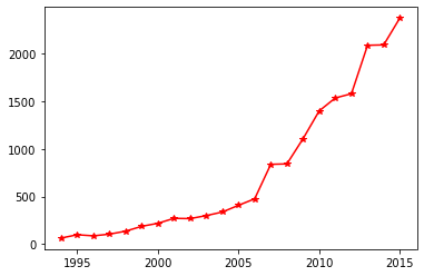
可视化操作 1 import matplotlib.pyplot as plt
1 2 plt.plot(y.index, y, 'r-*' ) plt.show()