0%

Python数据科学_15_案例:水色图像处理【简单计算机视觉】

读取图片数据

1
2
import os
import cv2
1
2
path = 'water_images'
imgname_list = os.listdir(path) # 获取path文件夹下所有的文件名称

数据集下载

1
2
3
4
5
6
7
8
9
imgs = []  # 用来存储每次读取到的图片数据
labels = [] # 用来存储每次计算得到的类别
for i in range(len(imgname_list)):
# 根据图像的文件名去获取水质
labels.append(int(imgname_list[i][0]))
# 读取每张图像的具体像素
imgpath = path + '/' + imgname_list[i]
img = cv2.imread(imgpath)
imgs.append(img)

数据预处理

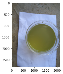
切分出每张图片的中心$100\times 100$区域图像

1
2
3
4
import matplotlib.pyplot as plt

plt.imshow(img[:, :, ::-1])
plt.show()

output_6_0_202303092118

1
2
3
4
5
6
7
# 1. 获取每张图片的尺寸
height, width = img.shape[:2]
# 2. 获取图像的中心点坐标
center_height, center_width = height // 2, width // 2
# 3. 根据中心点坐标获取中心点周围100x100的区域
new_img = img[center_height-50: center_height+50,
center_width-50:center_width+50, :]
1
2
plt.imshow(new_img[:, :, ::-1])
plt.show()

output_8_0_202303092118

1
2
3
4
5
6
7
8
9
10
11
12
# 按照上述操作,循环切分每张图片
new_imgs = []
for i in range(len(imgs)):
img = imgs[i]
# 1. 获取每张图片的尺寸
height, width = img.shape[:2]
# 2. 获取图像的中心点坐标
center_height, center_width = height // 2, width // 2
# 3. 根据中心点坐标获取中心点周围100x100的区域
new_img = img[center_height-50: center_height+50,
center_width-50:center_width+50, :]
new_imgs.append(new_img)
1
2
3
# 将列表转化为数组
new_imgs = np.array(new_imgs)
labels = np.array(labels)
1
new_imgs.shape
(197, 100, 100, 3)

计算每张图像的一阶矩、二阶矩和三阶矩数据

1
2
3
4
5
6
7
8
9
10
11
12
13
14
15
16
17
18
19
20
21
22
23
# 将三个通道分开
b, g, r = new_img[:, :, 0], new_img[:, :, 1], new_img[:, :, 2]

# 计算一阶矩
b_1 = np.mean(b)
g_1 = np.mean(g)
r_1 = np.mean(r)

# 计算二阶矩
b_2 = np.std(b)
g_2 = np.std(g)
r_2 = np.std(r)

# 计算三阶矩
def cal_3(array_):
E = np.mean(array_)
tmp = np.mean((array_ - E) ** 3)
result = np.sign(tmp) * (np.abs(tmp)) ** (1/3)
return result

b_3 = cal_3(b)
g_3 = cal_3(g)
r_3 = cal_3(r)
1
2
3
4
# Python内部默认是无法对负数求奇次方根
# 那么在对负数求奇次方根时,需要先将负数的符号取出
# 然后对其绝对值求奇次方根
(-8) ** (1/3)
(1.0000000000000002+1.7320508075688772j)
1
2
# 定义存储矩特征的容器
featues = np.zeros((len(new_imgs), 9))
1
2
3
4
5
6
7
8
9
10
11
12
13
14
15
16
17
18
19
20
# 循环计算所有数据的3阶矩
for i in range(len(new_imgs)):
new_img = new_imgs[i]
# 将三个通道分开
b, g, r = new_img[:, :, 0], new_img[:, :, 1], new_img[:, :, 2]

# 计算一阶矩
featues[i, 0] = np.mean(b)
featues[i, 1] = np.mean(g)
featues[i, 2] = np.mean(r)

# 计算二阶矩
featues[i, 3] = np.std(b)
featues[i, 4] = np.std(g)
featues[i, 5] = np.std(r)

# 计算三阶矩
featues[i, 6] = cal_3(b)
featues[i, 7] = cal_3(g)
featues[i, 8] = cal_3(r)
1
featues.shape
(197, 9)

数据集的切分(训练集+测试集)

1
2
3
from sklearn.model_selection import train_test_split

x_train, x_test, y_train, y_test = train_test_split(featues, labels, test_size=0.2)
1
2
print(x_train.shape)
print(x_test.shape)
(157, 9)
(40, 9)

训练模型和测试

支持向量机

1
from sklearn.svm import SVC
1
svm_model = SVC()
1
svm_model.fit(x_train, y_train)
SVC()
1
svm_model.score(x_test, y_test)
0.7

决策树

1
from sklearn.tree import DecisionTreeClassifier
1
tree_model = DecisionTreeClassifier()
1
tree_model.fit(x_train, y_train)
DecisionTreeClassifier()
1
tree_model.score(x_test, y_test)
0.875

神经网络

1
from sklearn.neural_network import MLPClassifier
1
mlp_model = MLPClassifier()
1
mlp_model.fit(x_train, y_train)
D:\Users\Python\Anaconda3.8\lib\site-packages\sklearn\neural_network\_multilayer_perceptron.py:692: ConvergenceWarning: Stochastic Optimizer: Maximum iterations (200) reached and the optimization hasn't converged yet.
  warnings.warn(

MLPClassifier()
1
mlp_model.score(x_test, y_test)
0.625

随机森林

1
from sklearn.ensemble import RandomForestClassifier
1
random_model = RandomForestClassifier()
1
random_model.fit(x_train, y_train)
RandomForestClassifier()
1
random_model.score(x_test, y_test)
0.95
模型名称 精度
支持向量机 0.7
决策树 0.875
神经网络 0.625
随机森林 0.95

从结果上来看,随机森林模型的精度达到了0.95,为4个模型中最高的一个,所以在解决该任务时,最好的分类模型是随机森林模型。

-------------本文结束感谢您的阅读-------------